In these online examples we show you how to draw wave families and calculate wave stability using the AUTO package. These instuctions will only work for those using UNIX/LINUX operating systems. You will also need to have AUTO properly installed on your computer. It can be obtained from http://indy.cs.concordia.ca/auto/. We used AUTO 97 to run these examples, which required us to modify the AUTO problem size restrictions. It appears as though newer versions of AUTO allow for larger problem sizes by default however we have not tested this. It is straightforward to recompile AUTO for larger problem sizes should you need to. Instructions to do this are in the AUTO manual (available at http://indy.cs.concordia.ca/auto/ ) under the heading "Restrictions on problem size". For your information we detail our own AUTO problem size limits in the file auto.h.
We give three different examples. We recommend that you perform these in numerical order.
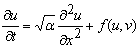
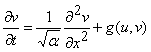
In this example we focus on the wave families of equations (2) of the main manuscript. To be explicit, in one space dimension these equations are:
| (A1a) | |
||
| (A1b) | |
where the variables u and v are the densities of predators and prey, respectively; t is time, x is the spatial coordinate, and α is the ratio of predator and prey dispersal coeffcients. The functions f and g are the predator and prey birth and death processes; we omit their full funcitonal forms here to improve the clarity of subsequent calculations but they are detailed in equations (2) of the main manuscript. The standard way of analysing travelling wave solutions of equations (A1) is to replace space and time by one coordinate that moves along with the periodic travelling wave. Here we use the travelling wave coordinate z=(x/c)-t, where c is the wave speed. This gives
| (A2a) |  |
||
| (A2b) |  |
where u(x,t)=U(z) v(x,t)=V(z) and prime denotes d/dz. This fourth order system of ordinary differential equations predicts stationary wave forms in the co-moving frame. Equations (A2) can then be written as a system of four first order ordinary differential equations in the standard way
| (A3a) |  |
||
| (A3b) |  |
||
| (A3c) |  |
||
| (A3d) |  |
Steady state solutions to this system are of the form (U,A,V,B)=(us,0,vs,0), with (us,vs) being the spatially uniform steady state solutions of the non-spatial predator-prey equations. Standard linear analysis of equations (A3) about these steady states reveals that the local stability of these steady states changes at a Hopf bifurcation wave speed. These steady state solutions are generally stable for speeds below cHopf but unstable for speeds greater than cHopf. This Hopf bifurcation point is the origin of the travelling wave families and can be calculated analytically (we omit the calculation here for brevity). Using the software package AUTO we can track the family of travelling wave solutions arising from cHopf in equations (A3) and study changes in the wave family shape caused by varying parameter values. AUTO is a software tool partly designed for continuation and bifurcation problems in ordinary differential equations. We wish to use AUTO for continuation. In other words, we can use it to locate a periodic solution (a periodic travelling wave) to equations (A3), and then track how the properties of that periodic travelling wave vary as we gradually change the equation parameters. We first use AUTO to compute the eigenvalues for equations (A3), with a given set of parameters and (U,A,V,B)=(us,0,vs,0), for c increasing through cHopf. This allows AUTO to detect cHopf. We then use AUTO to continue along the wave family arising from cHopf, for increasing c.
Click here to see an example of using AUTO to calculate the travelling wave families
Here we give examples of using AUTO to calculate the stability of travelling wave solutions. The methodology is considerably more complicated than above. Our approach is identical to that used by Smith and Sherratt (2007) and is described in general terms by them and in much more detail by Rademacher et al. (2007). However we give a broad overview here.
We wish to study whether small perturbations to periodic travelling wave solutions of equations (A1) will grow or decay. If they decay then the wave is locally stable, and if they grow then the wave is unstable. The standard approach to studying such stability is therefore to linearise equations (A2) about the periodic travelling wave solutions and then study their eigenvalues. However, rather than discrete eigenvalues, we are concerned with unbounded domains, for which there is an infinite spectrum of eigenvalues (Rademacher et al., 2007). Our intention is therefore to calculate this spectrum; if any eigenvalues have positive real part then we infer that the wave is unstable.
For the following calculations it is more convenient to use the alternative travelling wave coordinate z=x-ct. Substituting this into equations (A1) gives
| (A4a) |  |
||
| (A4b) |  |
||
| (A4c) |  |
||
| (A4d) |  |
We consider perturbations to equations (A1) of the form
| (A5a) |  |
||
| (A5b) |  |
where  ,
,  , and λ is an eigenvalue;
recall that (U,V) is the periodic travelling wave solution. Note that
, and λ is an eigenvalue;
recall that (U,V) is the periodic travelling wave solution. Note that  ,
,
 and λ are in general complex-valued
Substituting these solutions into equation (A1) and performing a Taylor expansion
gives the eigenfunction equations
and λ are in general complex-valued
Substituting these solutions into equation (A1) and performing a Taylor expansion
gives the eigenfunction equations
| (A6a) |  |
||
| (A6b) |  |
with boundary conditions
| (A7a) |  |
||
| (A7b) |  |
Here the subscripts on f and g denote their first derivatives with respect to u or v, calculated on the periodic travelling wave, and L is the wavelength. Boundedness requires that perturbations do not grow or decay in magnitude over each wavelength. However, there is no constraint on the phase change of the perturbation over a wavelength. Thus the appropriate boundary conditions are equations (A7), where γ can take any value between 0 and 2π. We need to obtain the eigenvalues for all possible phase shifts γ.
Stability analysis proceeds by first calculating eigenvalues corresponding to eigenfunctions that are periodic over one wavelength (γ=0), by discretising in z to give a (large) algebraic eigenvalue problem; we consider only eigenvalues with an appropriately large real part. The spectrum is then computed in AUTO by continuation of the real and imaginary parts of these eigenvalues as γ is increased from 0 to 2π. The continuation must be done starting separately from each of the eigenvalues calculated for the γ=0 case.
Click here to see an example of using this technique with AUTO to calculate the stability of three travelling waves on the wave family derived in the previous example.
Using the technique outlined above we can identify critical points in the wave family (such as a critical wavelength) at which the wave stability changes. In all cases we studied, wave stability changes through an Eckhaus instability at the origin in the eigenvalue complex plane. This means that the dominant perturbation grows monotonically in time, rather than having the form of growing oscillations. Mathematically, this is convenient as it allows us to perform numerical continuations in chosen parameters (e.g. α) to see how the position of the stability boundary varies. Specifically, we differentiate equation (A6) twice with respect to γ to give.
| (A8a) |  |
||
| (A8b) |  |
where | denotes d/dγ. This system of coupled differential equations includes the second derivative of the real part of the eigenvalue with respect to γ (λ||), zeros of which define Eckhaus points. We numerically continue the locations of these zeros to trace the stability/instability boundary for periodic waves. Further details of this procedure are given in Rademacher et al. (2007).
Click here to see an example of using this technique with AUTO to calculate how wave stability changes along the wave family and to trace the stability boundary.