>
CALCULATION OF NORMAL FORM FOR PREDATOR PREY SYSTEM NEAR HO PF BIFURCATION AND APPLICATION TO PERIODIC WAVES GENERATED BY AN OBSTACLE
INITIAL SETUPS FOR MAPLE
> restart;
> assume(A>1);
> assume(B>0);
> interface(showassumed= 0);
DEFINE THE EQUATIONS
> f:=q->q/(1+q);
![]()
> fp :=P*(A*f(H*C)-1)/(B*A):
> fh:=H*(1-H)-P*f(H*C):
(these are the nondimensionalised population kinetics terms: as in equation (A.3) in the paper)
STEP 2 IN APPENDIX OF PAPER: STEADY STATES AND LINEAR STABILITY ANALYSIS
> Hs:=solve(A*f(H*C)=1,H);
![]()
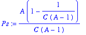
> Ps:=A*Hs*(1-Hs);
> tr:=1-2*Hs-Ps*C*subs(q=Hs*C,diff(f(q),q)):
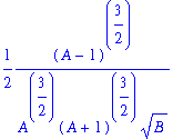
> Ccrit:=solve(tr=0,C);
![]()
> det:=C*Ps*subs(q=Hs*C,diff(f(q),q))/(B*A):
> real_evalue:=tr/2:
> imag_evalue:=sqrt(det-tr*tr/4):
> Lambda0:=subs(C=Ccrit,diff(real_evalue,C)):
> Omega0:=subs(C=Ccrit,imag_evalue):
> Omega1:=subs(C=Ccrit,diff(imag_evalue,C)):
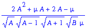
> simplify(Lambda0);
![]()
> simplify(Omega0);
![]()
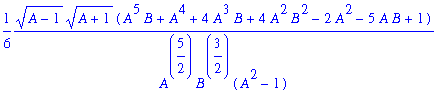
> simplify(Omega1);
NOW SET C=Ccrit
> C:=Ccrit:
> simplify(real_evalue); #CHECK ON VALUE -- SHOULD BE ZERO
![]()
> simplify(imag_evalue); #CHECK ON VALUE
![]()
STEP 3 IN APPENDIX OF PAPER: CONVERT LINEAR PART TO NORMAL FORM
> P:=Ps-phat*sqrt(A*(1-2*Hs)/B):
> H:=hhat+Hs:
> curlyF:=-fp/sqrt(A*(1-2*Hs)/B)+Omega0*hhat:
> curlyG:=fh-Omega0*phat:
NOW RUN SOME CHECKS ON curlyF AND curlyG -- there should be no linear terms
> simplify(subs(phat=0,hhat=0,curlyF));
![]()
> simplify(subs(phat=0,hhat=0,curlyG));
![]()
> simplify(subs(phat=0,hhat=0,diff(curlyF,phat)));
![]()
> simplify(subs(phat=0,hhat=0,diff(curlyF,hhat)));
![]()
> simplify(subs(phat=0,hhat=0,diff(curlyG,phat)));
![]()
> simplify(subs(phat=0,hhat=0,diff(curlyG,hhat)));
![]()
IF ALL SIX OF THE ABOVE GIVE ZERO, WE CAN CONTINUE.
STEP 4: CALCULATE LAMBDA1 AND OMEGA2
(using the formula given in the paper)
> Fpp:= subs(phat=0,hhat=0,diff(curlyF,phat$2)):
> Fph:= subs(phat=0,hhat=0,diff(curlyF,phat,hhat)):
> Fhh:= subs(phat=0,hhat=0,diff(curlyF,hhat$2)):
> Gpp:= subs(phat=0,hhat=0,diff(curlyG,phat$2)):
> Gph:= subs(phat=0,hhat=0,diff(curlyG,phat,hhat)):
> Ghh:= subs(phat=0,hhat=0,diff(curlyG,hhat$2)):
> Fppp:=subs(phat=0,hhat=0,diff(curlyF,phat$3)):
> Fpph:=subs(phat=0,hhat=0,diff(curlyF,phat$2,hhat)):
> Fphh:=subs(phat=0,hhat=0,diff(curlyF,phat,hhat$2)):
> Fhhh:=subs(phat=0,hhat=0,diff(curlyF,hhat$3)):
> Gppp:=subs(phat=0,hhat=0,diff(curlyG,phat$3)):
> Gpph:=subs(phat=0,hhat=0,diff(curlyG,phat$2,hhat)):
> Gphh:=subs(phat=0,hhat=0,diff(curlyG,phat,hhat$2)):
> Ghhh:=subs(phat=0,hhat=0,diff(curlyG,hhat$3)):
> Lambda1:=-(Fppp+Fphh+Gpph+Ghhh)/16+
> (Fpp*Gpp-Fhh*Ghh
> -Fph*(Fpp+Fhh)+Gph*(Gpp+Ghh))
> /(16*Omega0):
> Omega2:=(Gppp+Gphh-Fpph-Fhhh)/16+
> (Fpp*(Gph-Fhh)+Ghh*(Fph-Gpp)
> -3*Fhh*(Gph+Fhh)-3*Gpp*(Fph+Gpp)
> -2*(Fpp+Fhh-Gph)**2-2*(Gpp+Ghh-Fph)**2)
> /(48*Omega0):
> omega0:=(Omega0+mu*Omega1)/(mu*Lambda0):
> omega1:=-Omega2/Lambda1:
(Note: mu=C-C_crit)
END OF CALCULATION: NOW SIMPLIFY THE RESULTS
> simplify(omega0);
> simplify(omega1);
CHECK VALUES FOR VOLE - WEASEL PARAMETERS
> subs(A=1.8,B=1.2,omega0);
![]()
> subs(A=1.8,B=1.2,omega1);
![]()
NOW USE THE RESULTS TO TEST THE STABILITY OF PERIODIC TRAVELLING WAVES
GENERATED BY INVASION (WHEN MU=0)
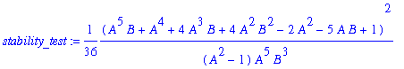
> stability_test:=simplify(omega1**2);
> # Wavetrain is stable iff stability_test<1.233
NOW VISUALISE THE STABLE/UNSTABLE PARAMETER REGIONS
(stable means stable periodic waves generated by bc;
unstable means spatiotemporal chaos generated by bc).
> with(plots):
Warning, the name changecoords has been redefined
> istable:=0: iunstable:=0:
> Amin:=1.01: Amax:=6.9: Bmin:=1.01: Bmax:=10:
> npoints:=30: Astep:=(Amax-Amin)/(npoints-1): Bstep:=(Bmax-Bmin)/(npoints-1):
> for aa from Amin to Amax by Astep do
> for bb from Bmin to Bmax by Bstep do
> if eval(subs(A=aa,B=bb,stability_test))<1.233 then
> istable:=istable+1:
> Astable[istable]:=aa:
> Bstable[istable]:=bb
> else iunstable:=iunstable+1:
> Aunstable[iunstable]:=aa:
> Bunstable[iunstable]:=bb
> fi
> od
> od:
> stablepoints:={seq([Astable[i],Bstable[i]],i=1..istable)}:
> unstablepoints:={seq([Aunstable[i],Bunstable[i]],i=1..iunstable)}:
> stableplot:=pointplot(stablepoints,color=red,symbol=circle,thickness=2):
> unstableplot:=pointplot(unstablepoints,color=blue,symbol=box,thickness=2):
>
neutrallystableplot:=implicitplot(stability_test=1.233,A=1.01..6.9,B=1.01..10,
color=green,thickness=3,numpoints=1000):
> unassign('ps');
> finalplot1:=display({stableplot,unstableplot,neutrallystableplot},
> labels=["A","B"],title="CIRCLE=stable, BOX=unstable"):
> plotsetup(default):
> finalplot1;
![[Maple Plot]](mapleworksheet21.gif)
THE END